Hyperparameter Tuning is just a Resource Scheduling Problem
When you hear hyperparameter tuning, you might think of trying lots of different model settings to find the best one—maybe using grid search, random search, or some fancy algorithm. But when you’re doing this at scale, especially with limited time or compute, it’s not just about finding the best settings. It’s about how you manage your resources. You have a bunch of models to try, but you can’t run them all fully.
So, the real problem becomes: given your limited computer power, which sets of settings should you even bother trying? For the ones you start, which ones should you stop early if they don’t look promising? And which ones seem good enough that you should give them more time and resources to see how well they can really do?
That’s exactly what some advanced tuning methods like ASHA, Hyperband, and Population-Based Training do constantly. They are making decisions about starting, stopping, and giving more power to different trials.
When you look at hyperparameter tuning this way, it stops feeling so much like a clever searching puzzle. Instead, it feels a lot like managing a list of tasks waiting to be done, where you have a limited budget of time and computer power. You have to decide which task to work on next, which ones to cut short if they’re not going well, and how to share your resources. That’s basically what a good scheduler does!
What is HPO ?
Hyperparameter optimization (HPO) is the process of choosing the best values for hyperparameters in a machine learning model. Hyperparameters are the settings or configurations that you decide before training the model. Examples include:
- Learning rate: How fast the model learns from data.
- Batch size: The number of training samples used to update the model’s weights at each iteration.
- Number of layers in a neural network
The space of possible hyperparameters is often vast, and the relationship between hyperparameters and model performance is typically non-linear and noisy. This means small changes in hyperparameters can lead to large fluctuations in performance.
Objective Function
The goal of HPO is to identify the set of hyperparameters that maximize (or minimize) some performance measure, usually the validation accuracy or loss of a model after training. This is typically expressed as an objective function.
$$\text{maximize} \ f(\theta) = \text{Accuracy}, \quad \text{or minimize} \ f(\theta) = \text{Loss}$$
The challenge lies in the fact that evaluating \(f(\theta)\) is often computationally expensive. It requires training a model with the specific hyperparameters \(\theta\) and then evaluating its performance on a validation set. This process can take hours or even days, especially when working with large datasets or complex models.
Example
Grid search is the most straightforward method. You define a grid of hyperparameter values, and the algorithm tries every possible combination. Let’s say you want to tune two hyperparameters: learning rate and batch size. You define the grid like this:
- Learning rates: 0.001, 0.01, 0.1
- Batch sizes: 32, 64, 128
The grid search will try all combinations:
- (0.001, 32)
- (0.001, 64)
- (0.001, 128)
- (0.01, 32)
- (0.01, 64) ………..
This approach is called exhaustive search because you are testing every possible combination, ensuring you explore all options. But here’s the catch: Grid Search is computationally expensive. If the model takes a long time to train (say hours), and you have more hyperparameters or larger ranges, the time to complete all combinations can quickly become impractical.
This is where resource scheduling comes into play, especially in large-scale tasks, where you need to decide how to allocate limited computational resources efficiently.
HPO as a Scheduling Problem
At a high level, hyperparameter optimization is about managing limited resources (like compute or time) and making decisions on which models to train, when to stop training them, and when to allocate more resources to the best-performing configurations.
Key scheduling-like aspects of HPO:
Limited Resources (Compute Budget):
Just like in scheduling problems, HPO algorithms are constrained by available resources. The more resources we can allocate, the more hyperparameter configurations we can test.
Evaluation Time (Task Duration):
Training a model with specific hyperparameters is time-consuming, like a long-running job in a job queue. Scheduling decisions are made on whether to keep running a long task or preempt it if other tasks seem more promising.
Exploration vs Exploitation (Job Allocation):
Exploration: Trying new or random configurations, akin to scheduling a new, untried job.
Exploitation: Allocating more resources to well-performing models, much like prioritizing jobs that are nearing completion and performing well.
Preemption & Job Promotion:
Early stopping (preemption) of low-performing models is equivalent to canceling jobs that aren’t worth the resources. Promotion happens when a model performs well in early trials and gets more resources, similar to scheduling more CPU time for the jobs that are performing best.
Advanced Algorithms: Scheduling HPO
These algorithms make the most efficient use of limited resources, helping us find the best hyperparameters faster. Let’s break them down.
ASHA
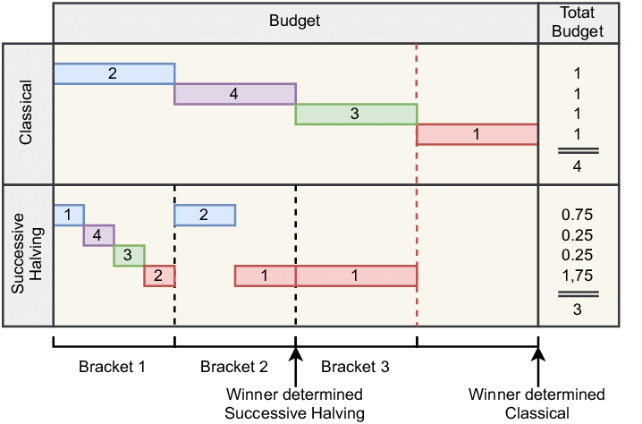
ASHA (Asynchronous Successive Halving Algorithm) is a highly efficient method for optimizing hyperparameters that focuses on allocating resources in a way that eliminates poor-performing models early, allowing us to concentrate computational power on the promising ones. It’s an enhancement of the traditional Successive Halving (SH) method, but with the added benefit of asynchrony, meaning we can evaluate multiple configurations in parallel, speeding up the process.
Initial Allocation: Each model starts with a small amount of resources, \( r_0 \).
$$ r_0 = \text{Initial Resources (e.g., 1 epoch)} $$
Subsequent Allocation: After each stage, allocate more resources to the remaining models.
$$ r_s = r_0 \times \eta^s $$
Where \( \eta \) is the scaling factor (typically 2 or 3), and \( s \) is the stage number.
Remaining Models: At each stage, the number of models is reduced by a factor of \( \eta \), i.e., only the top-performing \( \frac{1}{\eta} \) fraction of models are retained. $$ N * s = \frac{N*{s-1}}{\eta} $$
Hyperband
Hyperband is an enhancement of Successive Halving (SH) that allocates resources to different configurations in parallel, speeding up hyperparameter optimization (HPO).In the early stages, it explores the hyperparameter space with smaller resource budgets (Exploration), Later, it reallocates more resources to the best-performing models (Exploitation)
Parallel Successive Halving: Hyperband runs multiple SH processes in parallel with different initial resource budgets, exploring various configurations at different levels of commitment.
Resource Allocation: The resource for each stage \( s \) is calculated as:
$$ r_s = r_0 \times \eta^s $$
Where:
- \( r_0 \) is the initial resource,
- \( \eta \) is the reduction factor (e.g., 2 or 3),
- \( s \) is the current stage.
Resource Scaling: Resources grow exponentially at each stage. For example, if \( r_0 = 1 \) and \( \eta = 2 \):
- At \( s = 1 \): \( r_1 = 1 \times 2^1 = 2 \)
- At \( s = 2 \): \( r_2 = 1 \times 2^2 = 4 \)
- At \( s = 3 \): \( r_3 = 1 \times 2^3 = 8 \)
Trials Reduction: At each stage, the number of trials \( N*s \) decreases exponentially:
$$ N_s = \frac{N*{s-1}}{\eta} $$
Total Computational Budget: The total budget \( B \) is split across stages, where: $$ B = \sum_{s=0}^{S} r_s \times N_s $$ This ensures that more resources are allocated to the better-performing models as the process progresses.
Population-Based Training (PBT)
PBT is a more advanced method where multiple models (the “population”) are trained in parallel, and their hyperparameters are evolved over time. The idea is to explore hyperparameters and exploit good ones by periodically “mutating” hyperparameters of the best models and copying them to weaker models.
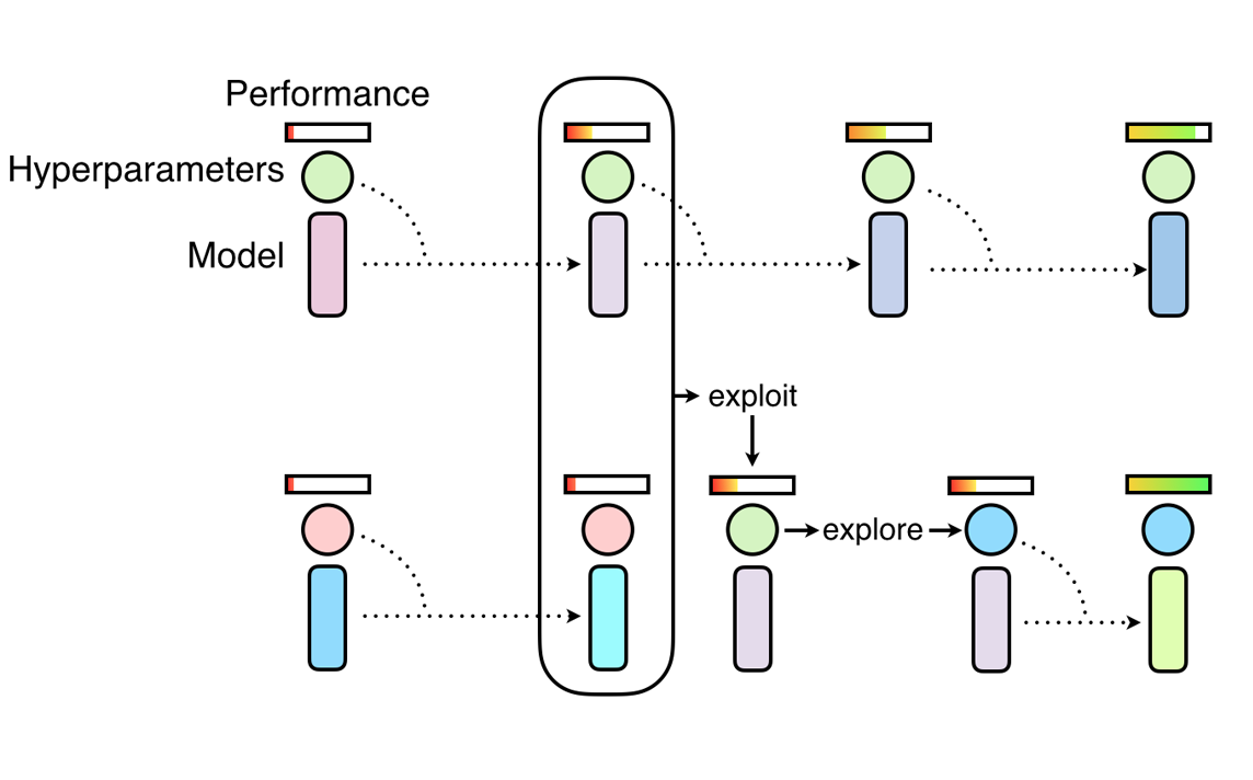
Typical Flow of PBT:
Initialization: The models are initialized with a set of random hyperparameters \( \theta_0 \).
$$ \theta_0 = \text{Random Initialization of Hyperparameters} $$
Evaluation and Selection: After training, models are ranked based on performance (e.g., validation loss). The best-performing models are selected:
$$ \text{Top Models} = { \theta^* } $$
Mutation: Hyperparameters of the top models are perturbed to create new configurations. $$ \theta_{\text{new}} = \theta^* + \Delta \theta $$ Where \( \Delta \theta \) is a random perturbation.
Comparison
| HPO Concept | ASHA | Hyperband | PBT |
|---|---|---|---|
| Resource Allocation | Allocates more resources to better-performing models | Similar to ASHA but with more exploration | Mutates best models, reallocates resources |
| Early Stopping | Eliminates poorly performing models early | Similar to ASHA | Evaluates and evolves the population of models |
| Exploration vs Exploitation | Explores a wide range, then exploits top models | Balances exploration and exploitation | Exploits best-performing models, mutates others |
| Scheduling Analogy | Job preemption, task prioritization | Job parallelism, dynamic scheduling | Task migration, job evolution |
Future Trends
- Meta-Learning: Meta-learning optimizes hyperparameters by learning from past optimization experiences, typically via optimization of a meta-objective function.
- Evolutionary Algorithms: Evolutionary algorithms like genetic algorithms are used for more adaptive search strategies. They simulate natural selection processes to iteratively evolve better-performing solutions
[2] Ray Scheduler